Filtered Vector Search: Why pgvector Returns Fewer Rows Than Your LIMIT
HNSW searches first and filters second. Here's how to tell which of your filters are losing results, and the fix for each zone.
Here's a query that looks completely safe:
SELECT id, content
FROM chunks
WHERE tenant_id = 42
ORDER BY embedding <=> $1
LIMIT 10;
Run it against a table with an HNSW index and it can return 4 rows. Or 2. Or none. No error, no warning, a fast and successful query that quietly ignored most of what you asked for.
This isn't an edge case someone found on a forum. pgvector's own README says that with approximate indexes, filtering is applied after the index is scanned, and gives the arithmetic: if a condition matches 10% of rows, with HNSW and the default hnsw.ef_search of 40, only 4 rows will match on average.
If your RAG system filters by tenant, user, permission scope, language, or document type, this is happening to some of your queries right now. The question is which ones.
TL;DR
- HNSW finds candidates by vector distance alone. Your
WHEREclause runs on whatever survives.- How bad it gets depends on selectivity (what share of rows match) and correlation (how close the matching rows are to the query).
- Narrow filters can go exact. Broad filters are fine. The middle loses results silently.
- Measure recall per filter bucket with an exact twin of each query, and alert on short results.
How post-filtering loses your rows
An HNSW index is a graph of vectors linked to their near neighbors. A search walks the graph toward the query and keeps a candidate list of size ef_search. When the list stops improving, the walk stops, and pgvector returns at most that many candidates.
The graph was built from vectors only. It has no idea what tenant_id is. So the sequence is:
- Walk the graph, collect the 40 nearest rows for everyone.
- Apply
WHERE tenant_id = 42. - Return whatever survived, up to 10.
If tenant 42 owns 10% of the table, spread evenly, about 4 of those 40 survive.
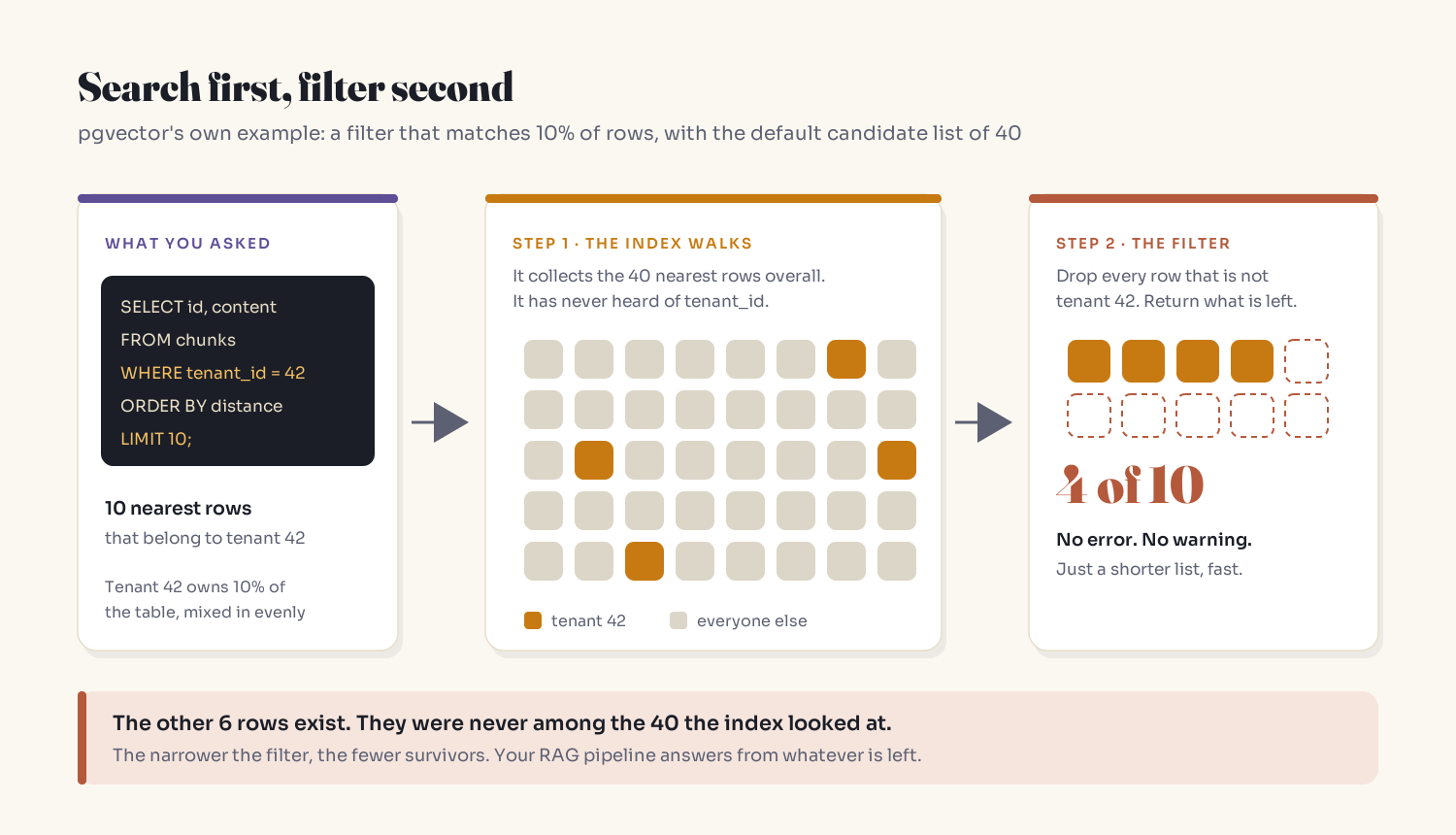
The six missing rows exist. They just weren't among the 40 the index looked at.
Three filtering strategies and how each one fails
| Strategy | How it works | Fails when |
|---|---|---|
| Post-filter | Approximate search, then drop non-matching rows | The filter is selective: too few candidates survive |
| In-graph filter | Skip non-matching nodes during the walk | Matches become disconnected "islands" in the graph, especially with combined filters |
| Pre-filter / exact | Find matching rows first, score every one | The filter matches a lot of rows: scoring all of them gets slow |
Qdrant's documentation describes the in-graph failure plainly: its filterable HNSW adds extra edges between points that share a value in an indexed payload field, but builds them per field, not per combination, so two or more strict filters can leave matching points disconnected and recall drops. Those edges are also only built for fields indexed when the graph is built. Index the field after ingestion and you need to rebuild the HNSW index to get them.
Selectivity decides which failure you get
Sort your filters by the share of rows they match and three zones appear.
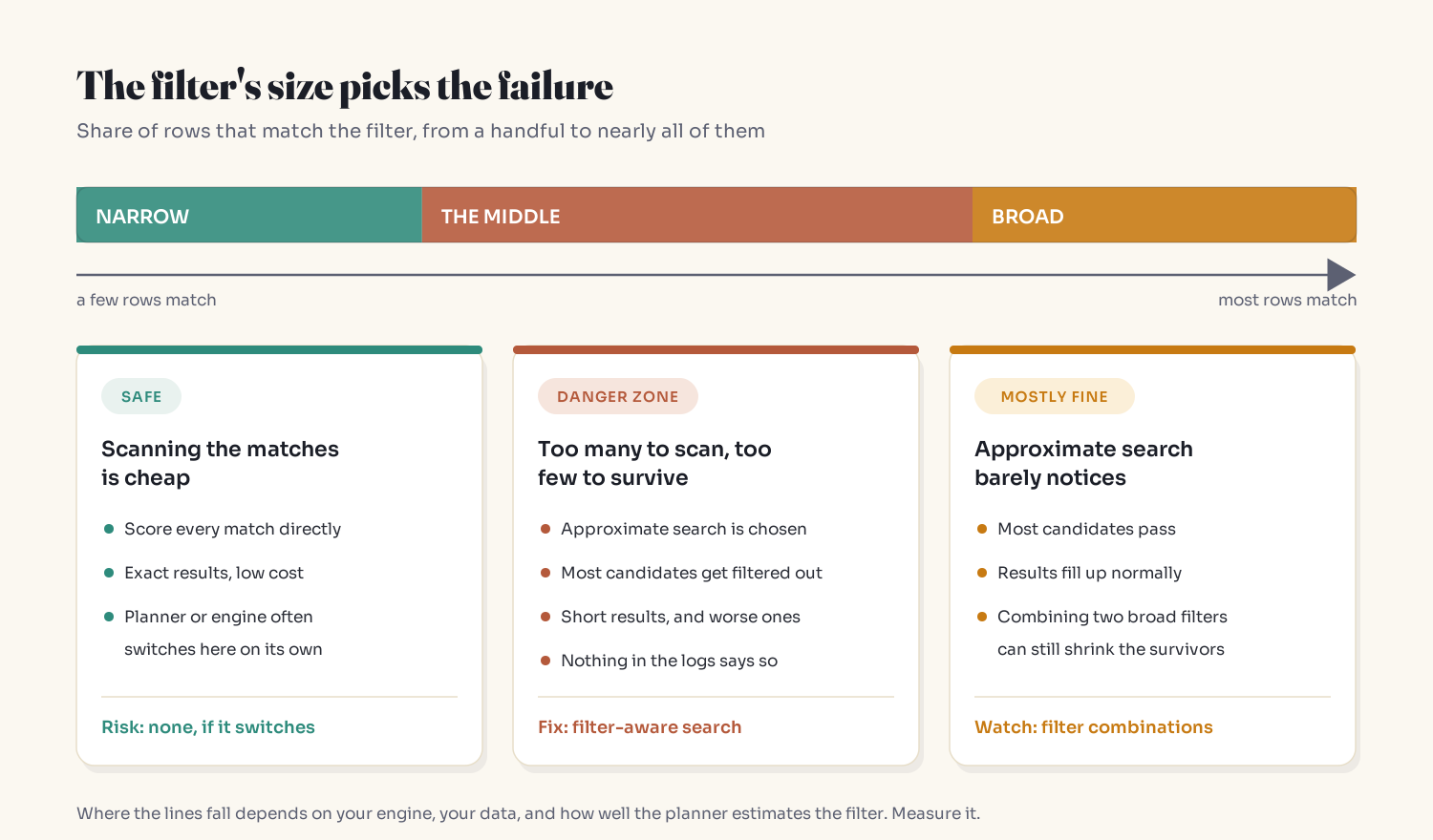
- Narrow. Few matching rows, so exact scoring is cheap and perfect. pgvector's README notes exact indexes work well for conditions matching a low percentage of rows. Qdrant switches to scoring each match directly below its
full_scan_threshold. - Broad. Most rows match, so most candidates survive. Mostly fine.
- The middle. Too many rows for the planner to choose exact, too few to survive post-filtering. Qdrant's docs single out mid-range matches with strict filters as the case where the graph can fall apart.
In a multi-tenant SaaS, the middle is your ordinary paying customer. Not the giant account you demo with, not the empty trial.
Correlation makes it worse
The "10% gives 4" math assumes matching rows are spread evenly. The ACORN paper (SIGMOD 2024) shows post-filtering performance depends on correlation between the query and the filtered set. When matching vectors sit far from the query, post-filtering can degrade toward a full scan.
Permission filters are the classic anti-correlated case. A finance user asks "how do deployment approvals work?" The nearest chunks company-wide are engineering runbooks they can't see. Their own approval policy is further out. Post-filtering returns nothing.
The Postgres planner adds a twist
Which path Postgres takes depends on the planner's row estimate for the filter. With prepared statements, Postgres may switch to a generic plan after a few executions, one built for a typical parameter value rather than this tenant (see plan_cache_mode). A small tenant can end up running the plan chosen for an average one. Check with EXPLAIN using real tenant IDs from each size bucket.
Fixing it in pgvector, zone by zone
Narrow: give the planner an exact path.
CREATE INDEX ON chunks (tenant_id);
The middle: iterative index scans (pgvector 0.8.0+). The scan continues until enough rows pass the filter or it reaches hnsw.max_scan_tuples (default 20,000).
BEGIN;
SET LOCAL hnsw.iterative_scan = relaxed_order;
SET LOCAL hnsw.max_scan_tuples = 40000;  -- tune per workload

WITH relaxed AS MATERIALIZED (
  SELECT id, content, embedding <=> $1 AS distance
  FROM chunks
  WHERE tenant_id = 42
  ORDER BY distance
  LIMIT 10
)
SELECT * FROM relaxed ORDER BY distance + 0;  -- + 0 needed on Postgres 17+
COMMIT;
relaxed_order gives better recall but can return results slightly out of order. The materialized CTE re-sorts them, which is the pattern pgvector's README shows. Use strict_order if you'd rather have exact ordering from the scan itself.
Do the arithmetic on the cap. A tenant owning 0.01% of a 10M-row table has 1,000 rows. Visiting 20,000 tuples, spread evenly, finds about 2. Iterative scans rescue the middle; the tiniest tenants still need the exact path.
Few or heavy filter values: partial indexes and partitions.
-- a few distinct values that matter a lot
CREATE INDEX ON chunks USING hnsw (embedding vector_cosine_ops)
WHERE (tenant_id = 42);

-- many values: partition, so big tenants get their own graph
CREATE TABLE chunks (
  id bigint, tenant_id int, content text, embedding vector(1536)
) PARTITION BY LIST (tenant_id);
Thousands of partitions carry their own operational cost, so this usually fits your heaviest tenants, with smaller ones sharing a default partition.
What not to do
Don't "fix" short results by dropping a permission filter from the SQL and filtering in application code after over-fetching. You've traded a recall bug for a data-exposure risk the first time a code path forgets the second step. Keep security predicates in the query.
The Exact Twin Test
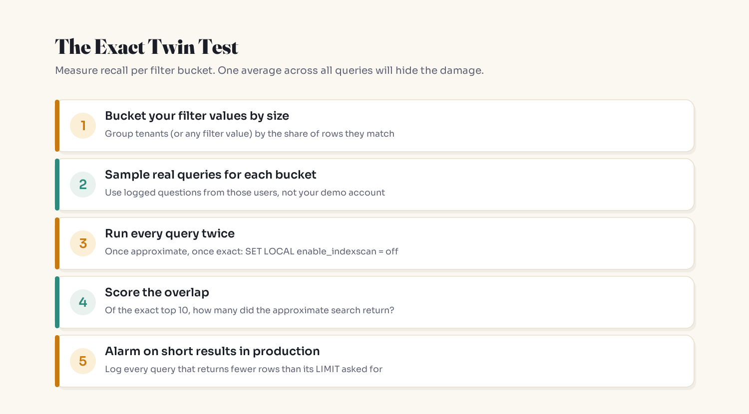
pgvector's README recommends monitoring recall by comparing approximate results with exact ones (SET LOCAL enable_indexscan = off). Do that, but per filter bucket:
import psycopg

QUERY = """
SELECT id FROM chunks
WHERE tenant_id = %(tenant)s
ORDER BY embedding <=> %(q)s::vector
LIMIT %(k)s
"""

def top_ids(conn, tenant, qvec, k=10, exact=False):
    """qvec is a pgvector literal string, e.g. '[0.12, -0.04, ...]'."""
    with conn.transaction():
        with conn.cursor() as cur:
            if exact:
                cur.execute("SET LOCAL enable_indexscan = off")
            cur.execute(QUERY, {"tenant": tenant, "q": qvec, "k": k})
            return [row[0] for row in cur.fetchall()]

def overlap_at_k(conn, tenant, qvec, k=10):
    exact = top_ids(conn, tenant, qvec, k, exact=True)
    approx = top_ids(conn, tenant, qvec, k)
    if not exact:
        return None  # tenant has no rows
    return len(set(exact) & set(approx)) / len(exact)
Run overlap_at_k over logged queries for tenants in each size bucket (tiny, small, medium, large) and report the mean per bucket. A healthy system scores similarly across buckets. If "medium" lags "large," you've found your middle.
Then add the cheapest production alarm you'll ever write:
def check_retrieval(rows, k, tenant_id, tenant_row_count, log):
    expected = min(k, tenant_row_count)
    if len(rows) < expected:
        log.warning(
            "short_retrieval",
            extra={"tenant_id": tenant_id, "asked": k,
                   "got": len(rows), "tenant_rows": tenant_row_count},
        )
Re-run the twin test when the table grows or a tenant moves buckets. Selectivity is a ratio; the zones move with your data.
Key Takeaways
LIMITis a ceiling, not a promise. Approximate vector search can return fewer rows than you asked for, with no error.- Post-filtering loses rows in proportion to how selective the filter is. pgvector's documented example: 10% selectivity,
ef_search40, about 4 rows. - Correlation matters: filtered rows that sit far from the query (permission filters are a classic case) do worst.
- Narrow filters should go exact, the middle needs filter-aware search (iterative scans, filterable indexes, partitions), broad filters are mostly fine.
- Measure recall per filter bucket with exact twins, and alert whenever a retrieval returns short.
- Never move permission filters out of the query to improve recall.
FAQ
Why does my pgvector HNSW query return fewer rows than LIMIT?
Because filtering happens after the index scan. HNSW returns at most hnsw.ef_search candidates (40 by default), and the WHERE clause removes the ones that don't match. If only 10% match, you get about 4. Enable iterative index scans (pgvector 0.8.0+) or give narrow filters an exact path.
What is the difference between pre-filtering and post-filtering in vector search?
Post-filtering runs the approximate vector search first and drops non-matching results, which is fast but loses results for selective filters. Pre-filtering finds matching rows first and searches only those, which is exact but gets expensive when many rows match. Many engines now filter during the graph walk or switch between strategies per query.
Does increasing hnsw.ef_search fix filtered vector search?
Partly. A larger candidate list means more rows survive the filter, but every query pays the extra cost and very selective filters can still come back short. Iterative index scans adapt per query instead of raising the cost globally.
How do I do multi-tenant vector search in Postgres?
Add a B-tree index on the tenant column so small tenants can use exact search, enable iterative index scans for mid-sized tenants, and consider partial indexes or list partitioning for your largest tenants. Then measure recall separately for each tenant size bucket.
How do I measure recall for filtered vector search?
Run each sampled query twice, once normally and once with SET LOCAL enable_indexscan = off to force exact search, and compute how many of the exact top-k the normal query returned. Report the result per filter bucket, because a single average hides the slices that fail.
Is it safe to filter vector search results in application code instead?
For relevance filters it's just inefficient. For permission or tenant filters it's risky: over-fetching without the filter and trimming in code means any missed step can expose another tenant's data. Keep security predicates in the database query.
Related reading
- RAG Explained: How to Make AI Actually Use Your Data: the pipeline this bug sits inside
- Your RAG Found the Right Chunk. The Chunk Forgot Where It Came From.: the other way retrieval fails quietly
- Why Your Database Is Ignoring the Index You Just Added: the planner decisions behind which path your query takes
- Why AI Confidently Lies to You: what the model does with the rows that never arrived
- New here? Start Here: A Plain-English Map to Understanding AI
Get one of these in your inbox each week: subscribe to the Simply Explained newsletter.
The bottom line
A filtered vector search is two questions: what's closest, and what's allowed. An approximate index has only studied the first one. Know which zone each filter lives in, give it the strategy that zone needs, and measure where averages can't see.
Your vector search doesn't have a recall number. It has one per filter value.
Adam Jaber is a software engineer who writes Simply Explained: complex topics, made simple. No jargon, no hype.
About the author
- I'm a senior software engineer. I write Simply Explained, a plain-English breakdown of how AI and software actually work, and the quiet ways they break: AI fixes that hide bugs, agents that pick the wrong tool, health checks that take down healthy servers. One symptom, one analogy, one fix per piece. New here? Start with the pinned Start Here guide, or get one breakdown a week by email.
Comments
Join the discussionNo comments yet. Be the first to comment.